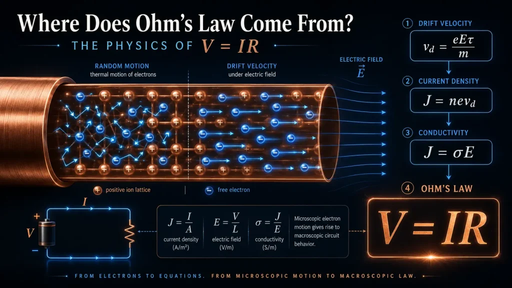
Ohm’s Law isn’t a starting assumption; it’s a consequence of how electrons actually move through a metal. This article derives V = IR from the physics of electron motion itself, using the Drude model, the same framework physicists use to explain why metals conduct electricity the way they do.
If you haven’t read the plain-language version yet, start with What Is Ohm’s Law? This piece goes underneath that one, into the mechanism.
The Physical Picture: Electrons in a Metal
A metal contains a huge number of free electrons that can move through the fixed lattice of positive ions. In copper, for instance, roughly one electron per atom is free to move; everything else stays locked to its atom.
Without an applied voltage, these free electrons move constantly in random directions due to thermal energy, colliding with the lattice roughly every 10⁻¹⁴ seconds. Because the motion is random, there’s no net flow of charge in any direction, no current.
Apply a voltage, and an electric field appears inside the wire. That field pushes every free electron in the same direction, superimposed on top of their random thermal motion. This small, consistent push in one direction is called drift velocity, and it’s the entire physical origin of electric current.
Deriving Ohm’s Law From Electron Motion
Between collisions, an electron accelerates under the electric field, then loses that gained velocity at the next collision with the lattice, and this repeated cycle produces a steady average drift velocity.
The force on an electron in a field E is F = eE (using e as the magnitude of the electron’s charge). Over the average time between collisions, τ (the relaxation time), the electron picks up an average drift velocity:
v_d = eEτ / m
where m is the electron mass; this is the average net velocity in the field’s direction, even though each electron’s actual path is a chaotic zigzag of collisions.
Current density J, current per unit cross-sectional area, depends on how many charge carriers there are, how fast they drift, and how much charge each carries:
J = n × e × v_d
where n is the number of free electrons per unit volume. Substituting the drift velocity expression:
J = n × e × (eEτ/m) = (ne²τ/m) × E
That coefficient, ne²τ/m, is the material’s conductivity, σ. So:
J = σE
This is Ohm’s Law in its most fundamental form: current density is directly proportional to the electric field, with the material’s conductivity as the constant of proportionality. Everything else, including the familiar V = IR, comes from integrating this relationship over a specific wire geometry.
From J = σE to V = IR
For a uniform wire of length L and cross-sectional area A, the field and current density relate directly to voltage and current: E = V/L (the field needed to push charge across the wire’s length) and J = I/A (current spread over the wire’s cross-section).
Substituting into J = σE:
I/A = σ(V/L)
Rearranging for V:
V = I × (L / σA) = I × R
where R = L/(σA). This is exactly the resistance formula used everywhere in circuit design; resistance depends on the wire’s length, its cross-sectional area, and the material’s conductivity. A longer wire has more resistance; a thicker wire has less; a better conductor (higher σ) has less. Ohm’s Law in the familiar V = IR form falls directly out of the microscopic electron-motion picture once you integrate it over a real wire’s shape.
A Real Number: Copper’s Relaxation Time
Copper’s relaxation time, τ, works out to roughly 2.5 × 10⁻¹⁴ seconds, derivable from copper’s own well-established physical constants, not an assumed value.
Copper’s electron density comes from its atomic properties: density 8,960 kg/m³, molar mass 0.0635 kg/mol, one free electron per atom. Using Avogadro’s number, that gives roughly n ≈ 8.5 × 10²⁸ free electrons per cubic meter.
Copper’s measured resistivity is 1.68 × 10⁻⁸ Ω·m, so its conductivity σ = 1/resistivity ≈ 5.95 × 10⁷ S/m. Rearranging the conductivity formula (σ = ne²τ/m) to solve for τ:
τ = σm / (ne²)
Plugging in the electron mass (9.109 × 10⁻³¹ kg) and elementary charge (1.602 × 10⁻¹⁹ C) gives τ ≈ 2.5 × 10⁻¹⁴ seconds, meaning a free electron in copper collides with the lattice roughly forty trillion times per second. That’s the physical reality behind copper’s conductivity value, not just a number pulled from a table.
Why Electrons Crawl, but Electricity Feels Instant
Drift velocity in a typical current-carrying wire is remarkably slow, often under a millimeter per second, even while the electrical effect itself seems to travel almost instantly.
Take a 12 AWG copper wire (cross-sectional area roughly 3.31 mm²) carrying 10A. Current density J = I/A ≈ 3.0 × 10⁶ A/m². Using J = nev_d and copper’s electron density from above:
v_d = J / (ne) ≈ 3.0×10⁶ / (8.5×10²⁸ × 1.602×10⁻¹⁹) ≈ 0.22 mm per second
Individual electrons drift slower than a snail. What actually moves quickly is the electric field itself, propagating through the wire at a significant fraction of the speed of light; every electron along the wire starts drifting almost simultaneously, which is why a light switch feels instant even though no single electron travels the length of the wire in that time.
When This Model Breaks Down
The Drude model assumes a fixed, voltage-independent relaxation time τ and a fixed number of free carriers, n. That assumption holds well for ordinary metals under normal conditions, which is exactly why Ohm’s Law works so reliably for wires and resistors.
It stops holding in two important cases: superconductors, where the entire physical picture of collision-based resistance disappears below a critical temperature, and semiconductors like diodes, where the number and behavior of charge carriers itself depends on the applied voltage. Both are covered in depth in Why Superconductors Break Ohm’s Law and Why Diodes Don’t Follow Ohm’s Law.
The point form derived here, J = σE, also generalizes beyond simple uniform wires to any shape, in any direction, at any point inside a conductor. That generalization, and why it matters for real engineering problems the simple V = IR can’t handle, is covered in The Point Form of Ohm’s Law: J = σE.
For the everyday circuit calculations this derivation ultimately supports, the Ohm’s Law Calculator handles the V = IR form directly.
A very important note: Please bear in mind that mathematical terms that are bold show they are vector quantities. Unbolded are scalar quantities.